Statistics
Here we will learn some basics of statistics. In particular, you will learn:
- The difference between univariate and bivariate analysis.
- The difference between correlation and causation.
- What does it mean that an association is significant.
Univariate and bivariate analysis
What distinguishes univariate analysis from bivariate analysis? At the end, univariate analysis we have already seen more than one variable in examples like this one that includes:
- Life expectancy (
lifeExp) on the x axis. - Continent (
continent) on the fill aestethic.
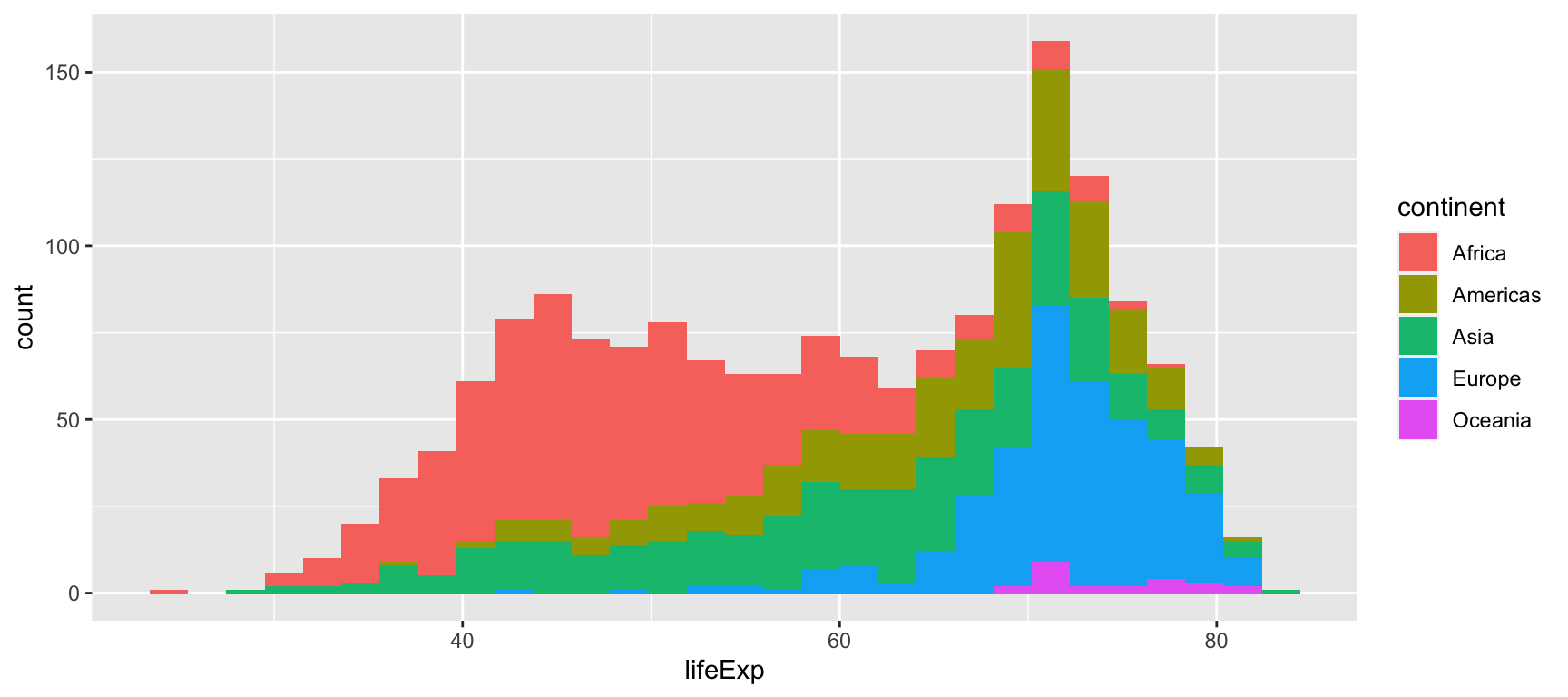
So, what is the difference between univariate and bivariate analysis? In short:
- Univariate analysis simply describes one (or more) variable(s).
- Bivariate analysis infers there might an association between two variables.
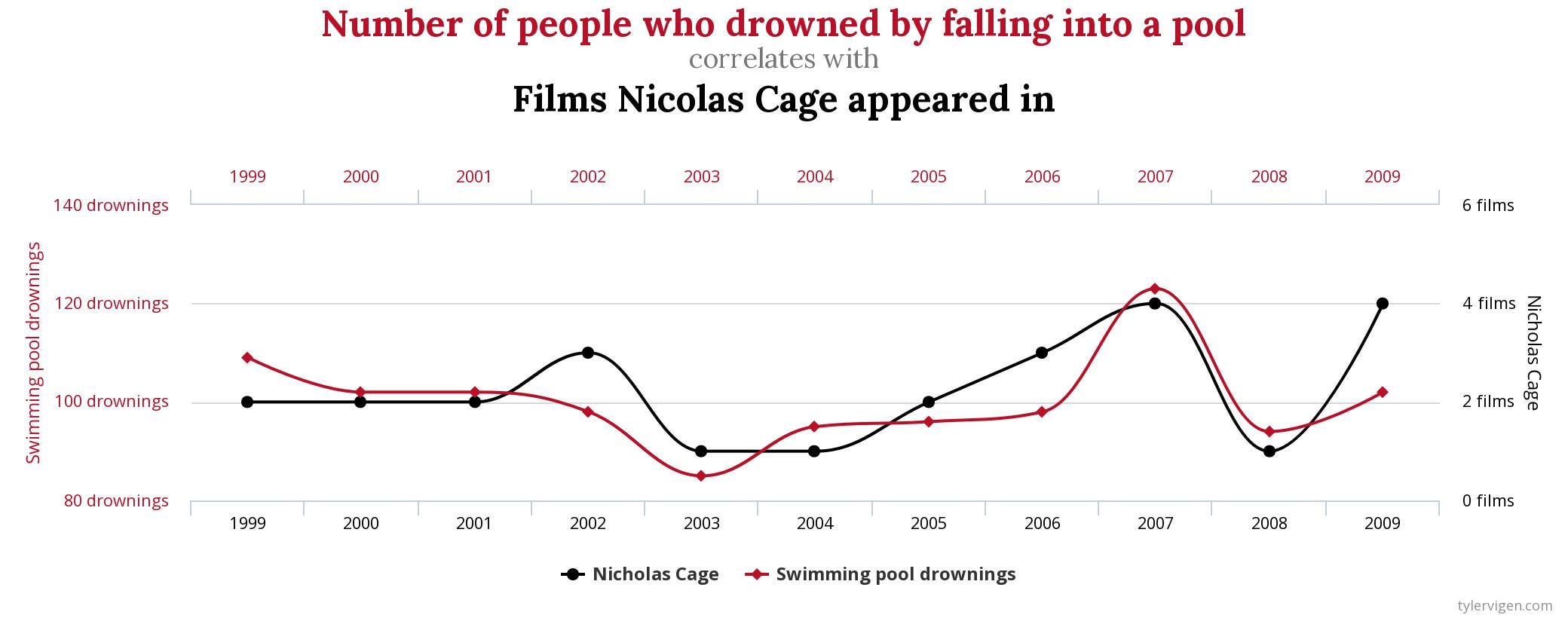
In the following examples, we won’t tell any lie if we simply describe the graph, but it will be silly to suggest some sort of causal association between variables:
- Figure 1: Pirates and global warming | Source: Wikicommons

- Figure 2: Nicholas Cage and number of drownings | Source: Miro Medium
- Figure 3: Paul the Octopus | Source: The Guardian

We have learnt two important things so far. First, that if we simply describe a graph we will never get in trouble. This is what univariate analysis does. By contrast, in bivariate analysis we enter to the realm of inferring associations between variables. Saying that one variable cause another is more problematic. As we have seen, correlation does not necessarily imply causation.
So, what do we need to say two variables are associated?
- Theory: The relation has to make sense.
- Correlation: Variables should vary together.
- Alternative variables: We should check other alternative explanations.
- Significance: We should see whether the relationship does not occur by chance.
Theory
Theory can be described as “what makes sense” to us. It is a logical reasoning that describes how to world (partially) functions. Wearing a silver coin in our left pocket may give luck to our football team. This is a (just) theory. Some people may think that the world functions in this way. Other people may believe that rich people tend to vote conservative. This is a (just) another theory. Theories have two requisites:
Temporality: The cause must be produced before or at the same time the effect happens.
- Climate and development
- New technologies and political polarization
Plausibility: It has to be somewhat reasonable.
- Age and conservative vote
Smart people do have strong theoretical knowledge. Normally these knowledge is acquired by reading a lot of books … although it is not the only way!
Tyrion Lannister quotes | Source: Hypable

Indeed, most of the things we know is because we are being told. But it is always good to do a double-check and look at the data.
Correlation
Once we know a relationship makes sense, we can test whether the relationship actually holds when looking at the data. For example, it might make theoretical sense to us that rural voters vote Donald Trump. People living in small towns are socially more conservative, preferring hence the conservative policies of the Republican Party than progressive policies of the Democratic Party. If our theoretical expectations are true, we expect that U.S. counties with low population are more likely to vote Trump. And indeed, as Figure 1 indicates, we observe a negative relationship between population size of the county and likelihood to vote Donald Trump in 20161.
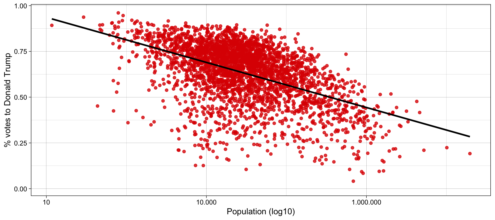
Figure 1: Votes to Donald Trump in every county (2016)
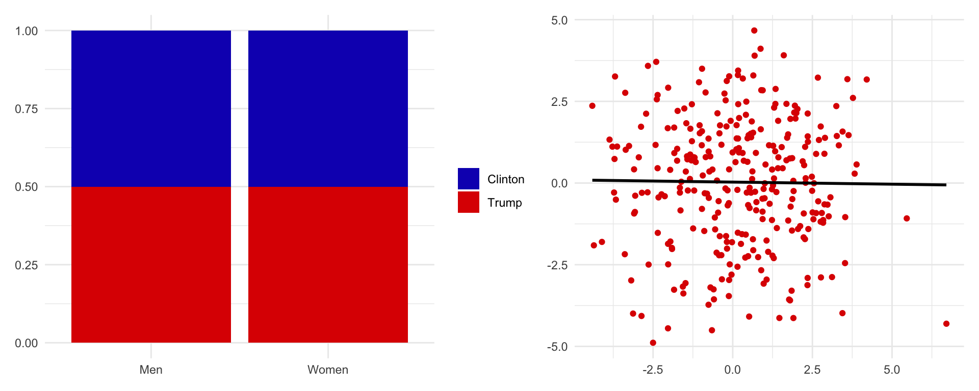
The previous figure seems to follow one of the necessary conditions for having association between variables: they are empirically related. This is, by knowing the value that takes one variable we can predict with more or less accuracy the value of the other variable. An important statistical test that we can conduct is to know how much they are related. If we look at the following hypothetical examples, it is clear that the relationship between sex and vote is stronger in the graph on the left than in the graph on the right.
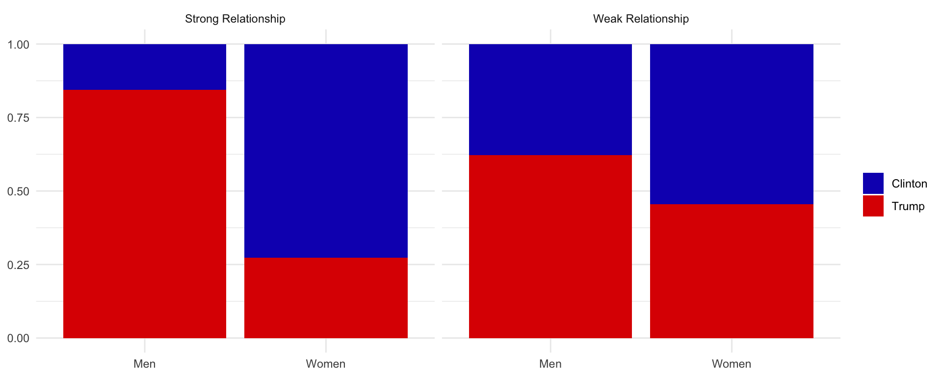
How much variables are related is called the strength of the relationship. The strength can be obtained by the association coefficient or the correlation coefficient (if we also want to know if the relation is positive or negative).
When do two variables not vary? In these two examples, no correlation is observed between variables. On the left side, knowing the sex of the individual does not bring any information on voting. On the right side, knowing the value of X does not provide any information on the value of Y. In this cases, the line that best represents the relationship is flat.
By multiplying per two the correlation coefficient we can obtain the determination coefficient, i.e., the R2. This coefficient tells us the chances we will have to guess correctly the values of the one variable if we are told the value of the other variable. Or, more technically, the proportion of the variance in the dependent variable that can be explained from the independent variable.
Alternative variables
But, what if rural vote has nothing to do with voting Trump? That would imply that there is nothing in particular of living in the countryside that makes you more prone to vote Trump. Perhaps it is not the size of the county that matters, but because they are less educated. Or because they have less income. All these variables might make theoretical sense to us. And it turns out that low-income, uneducated people live in small counties. All these variables are also empirically related to voting Trump, as we see in Figure 2. Therefore, we can’t know exactly which variables are associated with voting Trump and which variables only seem to be associated, but their effects are cleared out once we take into account the effects of other variables.
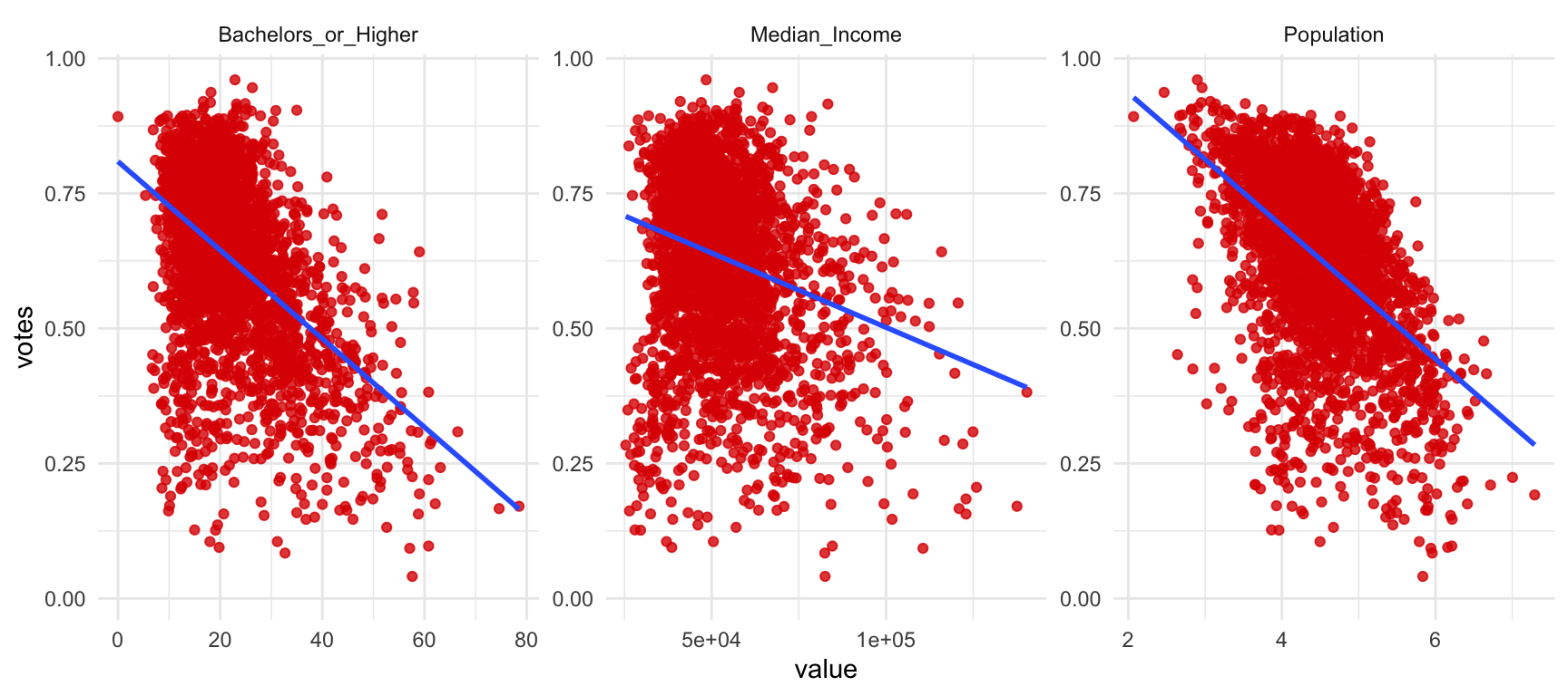
Figure 2: Alternative confounding variables
In the following Figure 3, we display the average results of an hypothetical Data Analysis course. On average, women seem to have high marks than men. On the basis of these results, we could infer that there is an effect of sex on the results. Women, due to some intrinsic characteristics, get better marks than men. Would we be right?
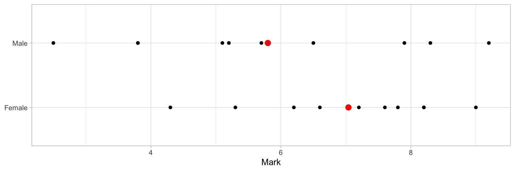
Figure 3: Scores in the Data Analysis course
Causal inferences are always stronger if we control for alternative explanations. What if … is there another variable that better explains why students in Data Analysis course get good grades? In Figure 4 we observe that, when controlling for the number of hours studied, the sex effects seem to disappear. Therefore, work discipline
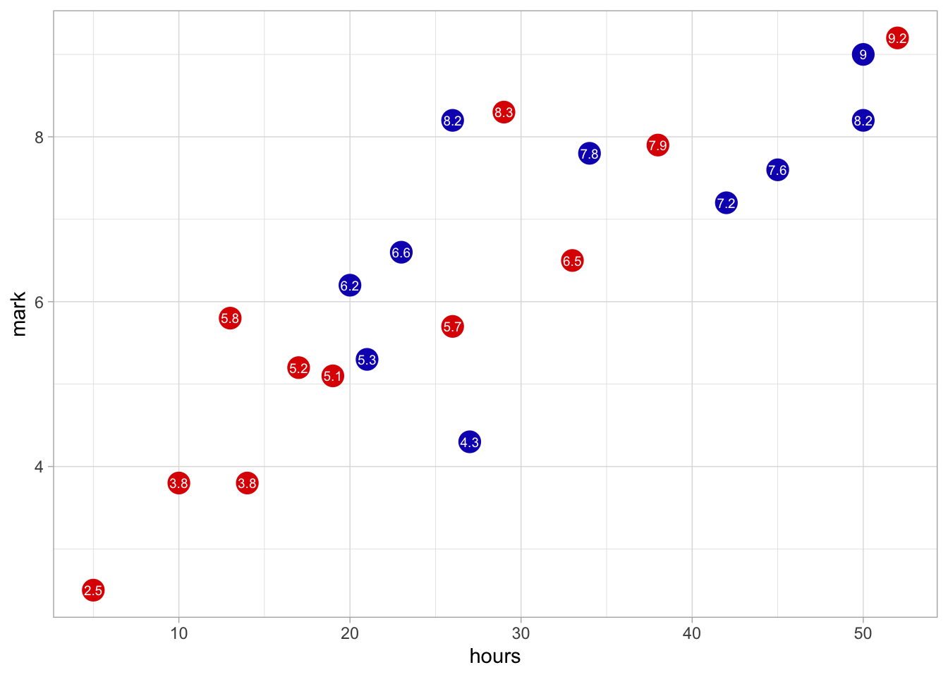
Figure 4: Mark by study hours
A golden rule is to test our hypothesis against other alternative confounding variables. This can we done with multivariate analysis.
Significance
Finally, in order to argue that two variables are related we must be sure that the relationship is not occurring by chance. Look at the following example. We randomly asked 60 people whether they voted Clinton or Trump. 29 responded they voted Clinton, whereas 31 responded they voted Trump. How likely it is that our sample can be generalizable to all U.S. population?
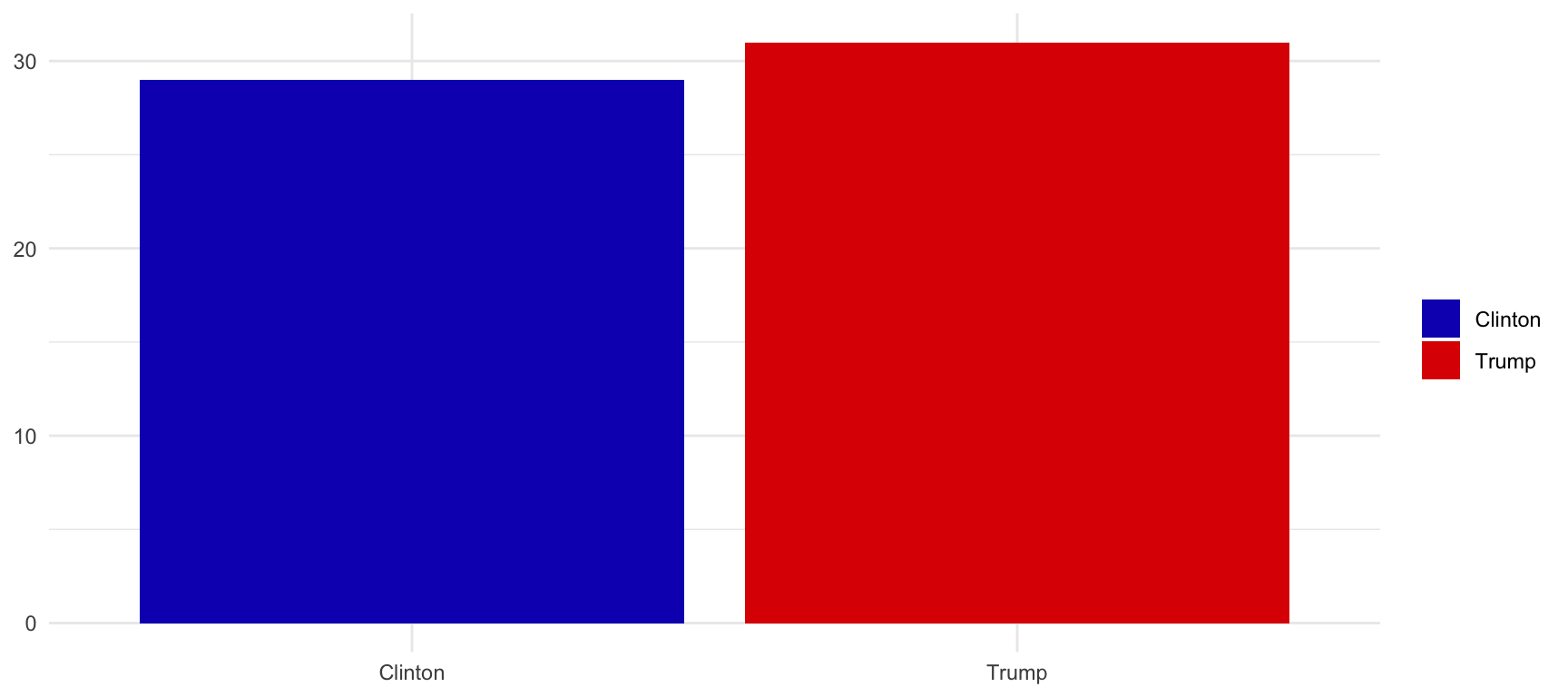
The answer is: not very likely. It is perfectly possible that the next two surveeyes will answer Clinton. Even that the next three will answer Clinton, shifting our predictions to a Democratic advantage. In order words, we cannot be very convinced that what we observe has not occurred by chance.
A similar parallel can be drawn when we flip a coin. If we flip it ten thousand times, we would expect that, around 5.000 we will get tails, and around 5.000 we will get heads.
table(sample(c("HEADS", "TAILS"), 10000, replace = TRUE))| Var1 | Freq |
|---|---|
| HEADS | 4940 |
| TAILS | 5060 |
So, what is the threshold that allows us to say confidently that the observed results are significant enough to not be produced by chance? Well, social scientists have agreed by convention that this point is when there is less than one to twenty (5% chance) to reject the opposite argument. If we observe that our hypothesized results have less than 5% (p-value below 0.05) to be produced randomly, then we can be confident enough about our argument. In statistics, testing how randomly are our results is called the significance test.
A significance test when we flip a coin would go as follows:
- I suspect that the coin has something weird and it must be tricked. I expect (my hypothesis) that I will get Heads too much times if I flip the coin several times.
- I flip one and get Heads. Well, there is 50 percent chance to get Heads.
- I flip again and get Heads. There is 25 percent chance to get two Heads.
- I flip another time and get another Heads. There is 12.5 percent chance to get three Heads. It is unlikely, but it can happen.
- I flip again and get another Heads. There is 6.25 percent chance to get four Heads in a row. This begins to be suspicious …
- I flip a fifth time and I get another Heads. I can’t believe it! There is only 3.125 percent chance to get five Heads in a row. The coin must be tricked!
Flipping and flipping: The following code calculates the difference between Heads and Tails when we flip a coin 10000 times. Then, we do the same procedure 1.000 times more, so as we can obtain a vector with 1.000 observations. Each observation tells us the difference occurred by chance of flipping a coin 10.000 times. Then, we generate a histogram of these differences.
u <- 0
for(i in 1:1000) {
  u[i] <- diff(as.vector(table(sample(c("HEADS", "TAILS"), 10000, replace = TRUE))))
}
hist(u, breaks = 10)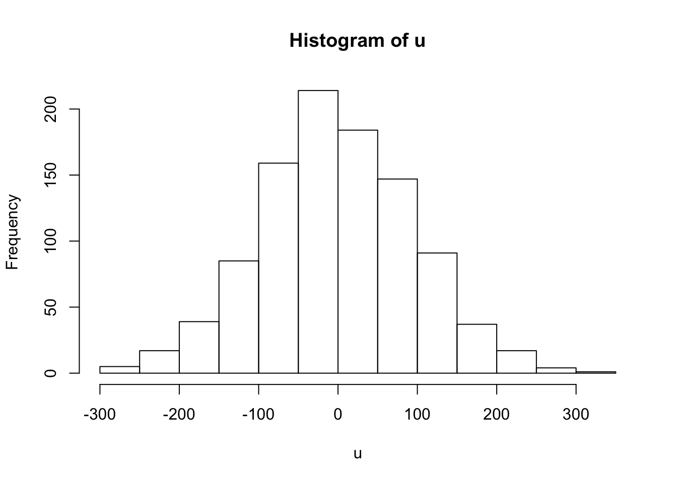
Look at the histogram. Is very likely to obtain a result that the difference between heads and tails is 50. However, it is very unlikely to obtain a difference above 200.
The significance test tells you, on the basis of your sample (five observations) and the obtained results (five Heads), how confident you can be to reject the opposite argument (the null hypothesis). If there is less than 5% chances, this is fair enough.
Significance test never tells you if you are right (it never does).
- It only tells you that you might not be wrong.
- Actually, it just says: well done, it looks good, keep doing more research on it!
Therefore, it is always good to read the results through confidence intervals to make inferences about the real world, especially when we deal with surveys:
Null hypothesis
The ‘opposite’ argument is called the null hypothesis. The null hypothesis is what we actually test in any scientific inquiry. As we can never be sure that what we say is true, what we can do is to argue how unlikely it is that the opposite would be true.
The null hypothesis is crucial in any scientific progress. Think of the following examples:
Ad Astra | Source: Pinterest

Robert O. Keohane
- “Although we are never likely to be able to predict or thoroughly explain specific strategic interactions among states, firms, and nongovernmental organizations, we can aspire to conditional generalizations that narrow the range of our uncertainty by accounting for general patterns of behavior” (Keohane 1997).
Oriol Mitjà
Fracasa el ensayo de Oriol Mitjà de usar hidroxicloroquina para prevenir la covid-19 https://t.co/rHKYCIjWdI
— EL PAÍS Catalunya (@elpaiscatalunya) June 11, 2020
Concluding remarks
“The crooks already know these tricks; honest men must learn them in self-defense” (Huff 1993, 9).
FOUR CARDINAL RULES OF STATISTICS 📈📊📉
— Daniela Witten (@daniela_witten) October 3, 2020
A thread
1/🧵